Finetuning DinoV3

Introduction

DinoV3 is the newest a foundation model for visual tasks released by Meta. It's a very powerful model that can be used as a backbone (or a feature extractor) for many downstream vision tasks, such as classification, segmentation, and depth estimation. By extracting visual features, it removes the burden when training our own models to learn them, streamlining the development of task-specific neural networks with state-of-the-art performance.

DinoV3 is originally trained with the LVD-1689M dataset, a Meta-owned dataset containing over 1B "public Instagram images," capable of generating high-quality features for real world images. While the base model performance may be great for real-world scenarios where it was trained, applying these features to other domains where the image patterns, colors, and textures are different from the training data can result in not-so-informative features. In this context, fine-tuning can significantly improve the performance.

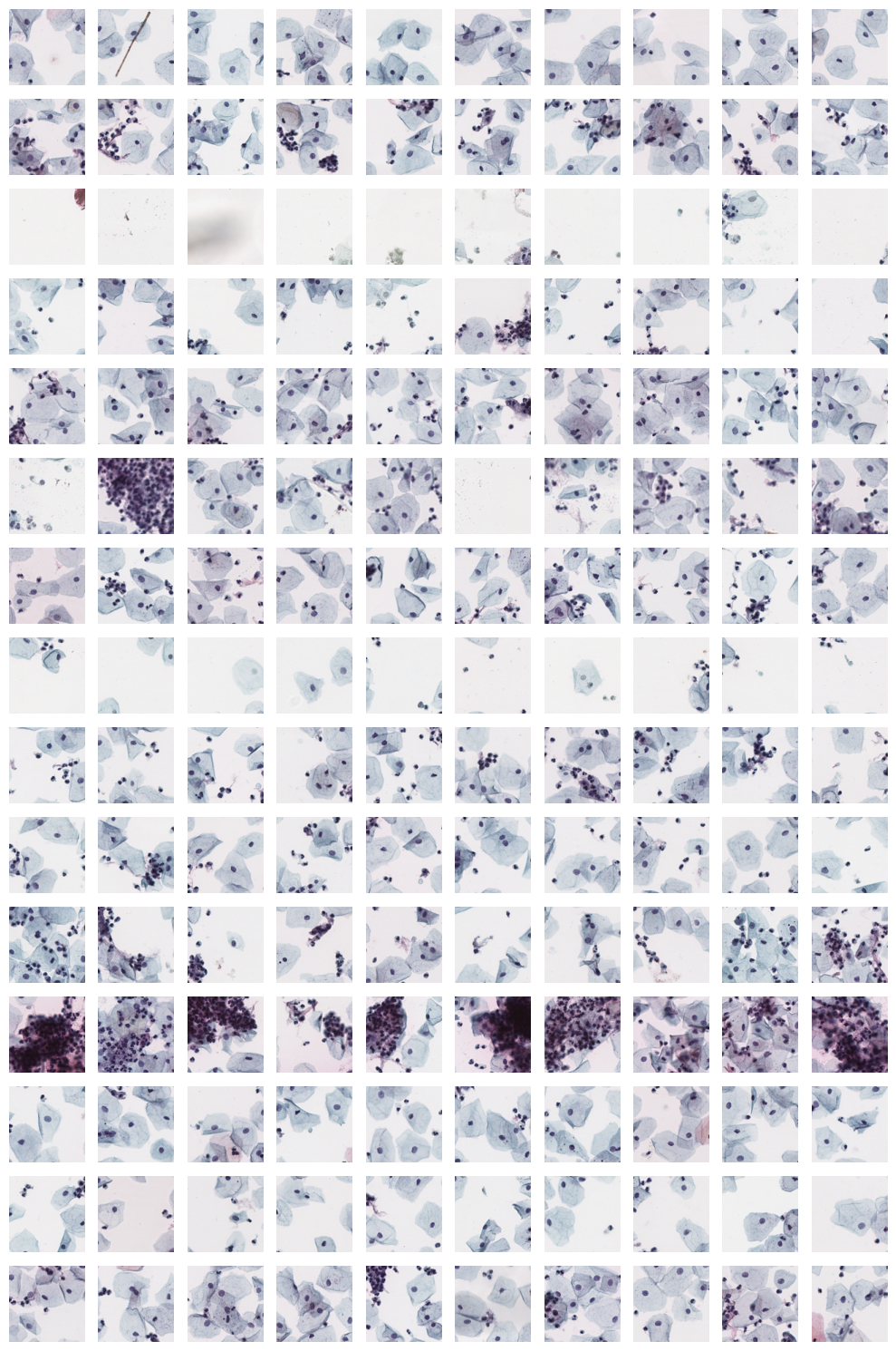
An example is my application domain: cytologic images classification, illustrated in the image below. It is quite different from the real-world image domain the DinoV3 is originally trained, and the images contain particular morphologies, staining patterns, and arrangements that we would like to be reflected in the features generated by the model.

In this post, I'll describe how to fine-tune the DinoV3 model using a custom dataset, along with the challenges I encountered during the process. This may be helpful for those who need to fine-tune the model with their own data, as the official repository lacks detailed implementation guidance for custom datasets and training from scratch.

Getting started

We start by cloning the project from the official GitHub repository.

git clone https://github.com/facebookresearch/dinov3.git

Then, instantiate your environment using your favorite management tool. For instance, with mamba:

mamba env create -f conda.yaml
mamba activate dinov3

The project might be overwhelming at first, but there are only a few directories we must get acquainted to inside the DinoV3 folder:

• configs\train\: contains example yaml configuration files, we will use this to create our configuration file.
• data\datasets\: this is where we are going to define our dataset and load the images.

Defining your dataset

Inside the data\datasets folder is where datasets are defined. Create a new file for the name of your dataset, for instance, my_dataset.py. Inside it, define the basic dataset class structure, which should extend from the ExtendedVisionDataset class.

from .extended import ExtendedVisionDataset


class MyDataset(ExtendedVisionDataset):
    def __init__(self,
                 transform=None,
                 target_transform=None
                 ):
        super().__init__(transform, target_transform)
        # TODO: implement your logic for gathering the images
        self.images = []
        self.transform = transform

    def __getitem__(self, idx):
        # TODO: implement logic for loading the image using PIL
        # NOTE: must return a tuple containing the image (PIL.Image) and the label. 
        # You may return None if your dataset has no label data.
        image = self.images[idx]
        if self.transform is not None:
            image = self.transform(image)
        return image, None

    def __len__(self):
        # TODO: return the number of items in your dataset
        return len(self.images)

A basic dataset must implement the __getitem__ and __len__ functions, in a traditional PyTorch fashion. The __getitem__ function must return a tuple containing the PIL.Image and a label associated with the image. If you don't have any label information (as it was in my case), you may return None.

Once your custom dataset is completed, you need to register it in the data/datasets/__init__.py file to load it directly when importing data/datasets.

from .ade20k import ADE20K
from .coco_captions import CocoCaptions
from .image_net import ImageNet
from .image_net_22k import ImageNet22k
from .my_dataset import MyDataset  # <- there

Now we must inform the loader how to instantiate your new dataset class. Proceed to the data/loaders.py file, which is responsible for instantiating the datasets from the argument of the yaml configuration file. Search for the _parse_dataset_str function (lines 46 -- 74) and modify it so the class_ variable points to your newly created class based on the value of the name variable.

For example, to instantiate the MyDataset class when the dataset is MyDataset on the configuration file, modify the function as such:

from .datasets import ADE20K, CocoCaptions, ImageNet, ImageNet22k, MyDataset  # <- add your dataset to the import list

...


def _parse_dataset_str(dataset_str: str):
    tokens = dataset_str.split(":")

    name = tokens[0]
    kwargs = {}

    for token in tokens[1:]:
        key, value = token.split("=")
        assert key in ("root", "extra", "split")
        kwargs[key] = value

    if name == "ImageNet":
        class_ = ImageNet
        if "split" in kwargs:
            kwargs["split"] = ImageNet.Split[kwargs["split"]]
    elif name == "ImageNet22k":
        class_ = ImageNet22k
    elif name == "ADE20K":
        class_ = ADE20K
        if "split" in kwargs:
            kwargs["split"] = ADE20K.Split[kwargs["split"]]
    elif name == "CocoCaptions":
        class_ = CocoCaptions
        if "split" in kwargs:
            kwargs["split"] = CocoCaptions.Split[kwargs["split"]]
    elif name == "MyDataset":  # <- the name of your dataset on the configuration file
        class_ = MyDataset  # <- point the class_ variable to your dataset class (not an instance of it!)
    else:
        raise ValueError(f'Unsupported dataset "{name}"')

    return class_, kwargs

Your custom dataset is now completed.

Defining your model

To train DinoV3 on your dataset, we must create a yaml configuration file defining your model and dataset, then start the training process. Training DinoV3 is divided in several steps, but for our use-case only the first two are really of interest: pretraining and gram anchoring.

Pretraining

Proceed to the config folder, we are going to set up the model. There are several files there already that will serve as examples of how to configure different parts of the training. We will start by the pretraining phrase, so make a copy of the dinov3_vit7b16_pretrain.yaml file.

Defining your dataset

Let's modify the original pretraining configuration for our needs. For starters, we will set the dataset to our newly implemented dataset class. Proceed to the train key and modify the dataset_path to use the name you set up on the loaders.py:

...
train:
  batch_size_per_gpu: 16
  dataset_path: "MyDataset"
  saveckp_freq: 20
  ...
  num_workers: 10

While you are there, there are several fields of interest that you might want to customize, such as the batch size, the save frequency, or the number of workers.

Defining your model

The key benefit of DinoV3 is that the proposed training enhancements allowed for scaling the model to 7 billion parameters, achieving a size comparable to popular large language models. The default training configuration proudly shows that. However, it's quite inviable for many people to train such a large model.

Luckily, similar to DinoV2, you can change the architecture of the network to a smaller one. Proceed to the student key, which defines the architecture of both the student and teacher networks. In my case, I used the vit_base model by changing the arch value:

...
student:
  arch: vit_base
  patch_size: 16
  ...

Other possible values include:

Continuing from LVD-1689M

The last modification of interest is to use the publicly available weights to continue the training rather than starting from random weights. Go to the Meta DinoV3 downloads website to request access and download the version compatible with the architecture you just selected.

Once you have access, download the model set its location within the MODEL key of the configuration file (the first key):

MODEL:
  META_ARCHITECTURE: SSLMetaArch
  DEVICE: cuda
  WEIGHTS: 'dinov3_vitb16_pretrain_lvd1689m-73cec8be.pth' # <- in my case vit-b, patch size of 16
  DTYPE: float32

Finally, the last field of interest is in optim. You may want to customize the epoch and perhaps the learning rate.

...
optim:
  epochs: 1000
  optimizer: adamw
  weight_decay: null
  weight_decay_end: null
  lr: null
  warmup_epochs: null
  min_lr: null
  ...

Launch the training

Now everything should be good to go! There are several ways to start training depending on your configuration. The recommended way is to use Meta's submitit library to control SLURM in your multi-node GPU cluster. If this is your case, you can follow the instructions of the official GitHub page and start training with the following command:

 PYTHONPATH=${PWD} python -m dinov3.run.submit dinov3/train/train.py \
  --nodes 4 \
  --config-file dinov3/configs/train/MyDatabase-pretrain.yaml \
  --output-dir MyDatabaseResult

However, if you don't have multiple nodes, or don't have a SLURM setup, you can start training on a single machine containing N GPUs by the traditional way: using torchrun. For this purpose I made the following run.sh file for launching the training.

#!/bin/bash
export CUDA_VISIBLE_DEVICES=1,2,3
export PYTHONPATH=.

torchrun --nproc_per_node=3 dinov3/train/train.py\
    --config-file dinov3/configs/train/cito/pretraining.yaml \
    --output-dir ./results-cito-base

The setup works as follows:

• CUDA_VISIBLE_DEVICES: limits which GPUs the process is allowed to use. In this context, I have 4xNVIDIA A100 40GB, and I am allowing the model to use 3 of them, excluding the first one.
• PYTHONPATH: includes the current folder in the Python module search path;

Training starts with the torchrun command. The --nproc_per_node=3 dictates that I want the training to occur with 3 GPUs (specified with the CUDA_VISIBLE_DEVICES). Then, we have the python script with the training code, the configuration file you just made (--config-file) and the results dir (--output-dir) where the model is going to be saved.

Some additional information: once training starts, it saves a checkpoint each checkpointing.period. If training is restarted, it will continue from the last checkpoint. Furthermore, the code also keeps track of the existing checkpoints and only keeps the last checkpointing.max_to_keep checkpoints. Finally, each checkpointing.keep_every iteration, a new permanent checkpoint is saved, so if anything happens you can go back to it.

You are ready to start training! Run:

bash run.sh

Unexpectedly, the process is Killed

You start training, and after a few minutes watching the logs, you get the message that the process is killed. Indeed, running the process again and checking with htop, you verify that the RAM usage keeps increasing on each new iteration.

If this happens to you as well, the solution is actually simple: proceed to the train/train.py script which dictates how the model is trained. There, on line 434, you see the comment "Manual garbage collection," followed by the gc.disable() that turns off the GC. It seems the authors' idea was to manually trigger the garbage collection, both in line 436 and, during the training loop, on line 466.

Unfortunately, on my setup (a single DGX A100 machine, with 4xA100 40gb), that didn't work. The GC gets disabled, but the manual collection doesn't happen. While the collection command does freeze the process for a couple of seconds, the memory consumed by the previous iteration doesn't get released, and the whole process is killed after a few iterations.

Removing the command to disable and to perform the collection solves the issue. My intuition is that this approach doesn't work when using torchrun, or perhaps it's related to a single node training. Regardless, the removal of the instructions solves the Killed issue and allows the training procedure to continue as intended.

Gram anchoring

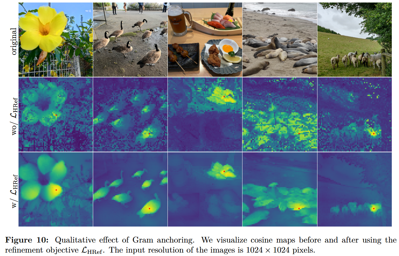
Now that the pretraining phrase is done, you might want to continue training with gram anchoring as well. Gram anchoring is one of the solutions that allow DinoV3 to scale the train procedure and enable the development of larger models. It uses an early checkpoint that has a supposedly stable dense feature to prevent the degradation of the dense feature introduced by longer training schedules. You can read about it in the paper.

To start the gram anchoring training, you must enable it in your configuration file. Check the configs/train/dinov3_vit7b16_gram_anchor.yaml for an example of how to set the key gram on your file to true. Replacing the entire object is a start.

Importantly, training requires the ckpt value to be set. This is the path to that "previous" checkpoint that will be used to produce stable dense features and guide the rest of the training. When I was first implementing this, it wasn't clear what this value was supposed to be, since pointing to a checkpoint inside the results folder wasn't working: it complained that the model keys were incompatible with what they expected.

The expected value is a checkpoint inside the eval folder (for example /MyDatabaseResult/eval/). Instead of using a full checkpoint containing both the teacher and student networks generated during training, you must point to a checkpoint containing only the teacher network that is generated periodically inside the eval folder on your output directory. Point the ckpt value to any checkpoint inside the eval folder and start the training again to continue the process with gram anchoring.

Training, tracking, and inferencing

During training, the logs, metrics, checkpoints, and configuration file is saved in the defined output folder. The folder has the following structure:

• eval: contains periodically saved teacher models;
• ckpt: contains the training checkpoints, including the teacher and student networks to resume training;
• logs: contains the text logs per GPU;
• config.yaml: contains the configuration file defining the model trained in this folder;
• training_metrics.json: contains the metrics in a JSONL format.

Let's explore what options those files enable during training and after training the model.

Tracking progress

DinoV3 logs the training metrics in a jsonl file inside the output folder, named training_metrics.json. This makes it quite easy to check the results using a jupyter notebook. For example, the following code should plot the total_loss:

import json
import pandas as pd
import matplotlib.pyplot as plt

with open("MyDatabaseResult/training_metrics.json", "r") as f:
    items = [json.loads(line) for line in f.readlines()]
    items_df = pd.DataFrame(items)

plt.plot(items_df.total_loss)

Inferencing and testing

During training, instantiating and playing with the model can also be done, both with the training checkpoints which are updated more frequently and the eval checkpoints. Let's explore how to instantiate and run inference with the model you are training.

Instantiating the model

The first step is to instantiate the model with your configuration file. For this purpose, the config.yaml file in your output directory is used, as it contains the parameters that describe how the model should be created, such as the number of parameters, allowing the saved weights to match.

The model can be instantiated from your config.yaml file using the build_model_from_cfg file from dinov3.models. Use the OmegaConfig library to load your yaml file:

from dinov3.models import build_model_from_cfg
from omegaconf import OmegaConf

cfg = OmegaConf.load("MyDatasetResult/config.yaml")
student, teacher, embed_dim = build_model_from_cfg(cfg)

The function returns a tuple containing the student network, the teacher network (generally used for inference) and the embedding dimension generated from the networks.

Loading the weights

Now we have a randomly initiated ViT, but it's still missing the weights we trained with our dataset. DinoV3, in contrast with DinoV2, uses the recommended Distributed Checkpoint (DCP) system to save the checkpoints while in multi-GPU environments, which uses file formats that can't be loaded with torch.load.

Luckily, DPC has a function to convert the checkpoint back to a serialized "torch" file:

from torch.distributed.checkpoint.format_utils import dcp_to_torch_save

dcp_to_torch_save("MyDatasetResult/ckpt/949999_keep", "MyResults.pt")

Now, the weights can be loaded as normally with the torch.load function:

import torch

checkpoint = torch.load("MyResults.pt", weights_only=False)

In the example below, we prepare and load the weights from the teacher network from a training checkpoint. Notice that the checkpoint contains both networks, so we create a new object and only add the weights of the teacher. Furthermore, we skip keys related to the gram network, and we also remove the "backbone." key for the keys to match the expected name:

model_weights = checkpoint["model"]

teacher_weights = {}
for key, value in model_weights.items():
    if "teacher.backbone" in key and "gram_" not in key:
        teacher_weights[key.replace("teacher.backbone.", "")] = value
teacher_weights.keys()

To instantiate the model on the first GPU with the correct weights, use the following code:

teacher = teacher.to_empty(device="cuda")
teacher.load_state_dict(teacher_weights, assign=True, strict=True)
teacher = teacher.to("cuda").eval()

You may want to serialize the model using ONNX for using it in the future.

Conclusion

I trained the model for a couple of days on 3xA100 GPUs and used the model to extract features for Multiple Instance Learning tasks in the cytology domain. While I am not ready to show the results we got, I can say that I am impressed by the performance and can atest to the benefits of fine-tuning DinoV3 when you need to use the model in a different domain from what it was trained.

To illustrate the results we got, I used the model for extracting features of the tiles from a given cytology slide. I then used PCA to turn the 738 features into three main components, which are used to color the different tiles. This allows us to have an idea of different or similar each tiles are from themselves.

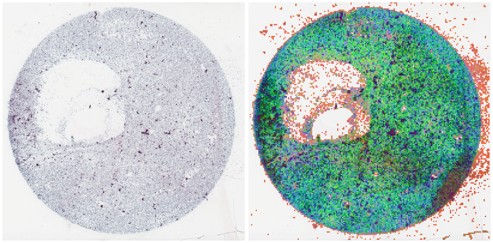
Notice, however, that those 3 main components only account for 18% of the distribution of features learned (a good sign!), signifying that each feature learned by our fine-tune of DinoV3 has unique information about the tile.